2 Hardware Solutions
2.1 Environmental Variables
2.1.1 NiMH Solar Trickle Charger
2.1.1.1 Purpose & Use Case:
The solar trickle charger module presented here is designed to provide a simple, low-cost, and field-deployable solution for recharging AA NiMH batteries in remote areas. Its primary use case is to support small-scale electronic devices—such as environmental sensors or data loggers—used in off-grid research and monitoring setups. Especially relevant in the Global South and other regions where access to stable electricity is limited, this charger enables reliable, low-maintenance battery recharging using solar energy. By leveraging basic components like a small solar panel and a Schottky diode, the system offers a practical way to maintain battery-powered devices in the field without the need for complex charging infrastructure or frequent battery replacement.
2.1.1.2 Bill of Materials:
A comprehensive overview of all components required to build the solar charger, needed quantities, recommended suppliers and approximate prices (in €) is provided in Table 2.1
| Component | Amount | Supplier | Price (approx.) |
|---|---|---|---|
| Shotky-Diode | 1 | Amazon, Reichelt, Conrad | 0.10 € |
| Common E-Series electronic resistor (e.g., 10 Ω) | 1 | Amazon, Reichelt, Conrad | 0.10 € |
| 6AA Battery holder | 1 | Amazon | 3.00 € |
| Perfboard / MonksHillLab PCB board (2x2 cm) | 1 | Amazon | 0.50 € |
| Wires (black, red) / Screw Terminal Blocks | – | Amazon | 0.50 € |
| 6V, 2.5W Solar Panel | 1 | Amazon | 10.00 € |
| Sum | 14.20 € |
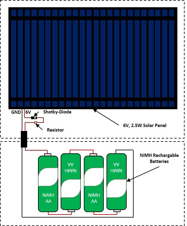
2.1.1.3 Wiring Diagram:
A schematic overview of the wiring layout, showing all necessary connections between electrical components, is provided in Figure 2.1.
2.1.1.4 Assembly Instructions:
- Solder a 5cm black and red wire to + and – pole of the solar panel.
- Solder two 2x2 Screw terminal block (screw terminal 1 to 4) on the tiny perfboard/PCB board.
- Remove 0,5cm isolation from the red wire coming from the solar panel and fix it in screw terminal 1.
- Connect screw terminal 1 (Anode) and 2 (cathode) using the shotky-diode.
- Connect screw terminal 2 and 3 using the 10 Ohm resistor.
- Connect screw terminal 3 with + of the 4AA battery holder (using a red wire).
- Remove 0,5cm isolation from the black wire coming from the solar panel and fix it in screw terminal 4.
- Connect screw terminal 4 with - of the 4AA battery holder (using a black wire).
- Seal solder connections using e.g. transparent nail polish.
2.1.1.5 Calibration:
Precise calibration is not required. To verify functionality, insert fully discharged NiMH batteries of the same type and capacity into the holder and expose the solar panel to direct sunlight for several hours. A gradual voltage increase indicates proper trickle charging. A current-limiting resistor (e.g., 10 Ω) is used to regulate charging current, based on Ohm’s Law (I = V / R). This ensures a safe, low current suitable for trickle charging, typically around 1/100th of the battery capacity per hour (e.g., 20 mA for 2000 mAh cells). The resistor value can be adjusted to suit panel output and battery size—higher resistance lowers the current to prevent overcharging in bright sunlight.
2.1.1.6 Code:
No specific code is provided for this module, as it operates passively without a microcontroller.
2.1.2 Photosynthetic Active Radiation (PAR) Sensor
2.1.2.1 Purpose & Use Case:
The PAR sensor module presented here can be used to determine photosynthetically active radiation (PAR), the range of solar radiation between 400 and 700 nm that is relevant for plant photosynthesis. While this chapter focuses on the construction and calibration of the sensor itself, it is designed to be integrated into larger monitoring setups that include power supply and data logging via a microcontroller. The sensor module thus serves as a Component in more comprehensive systems—such as automatic climate stations or gas flux chambers described in later chapters—where continuous PAR measurements are essential for understanding environmental conditions and light-driven plant processes.
2.1.2.2 Bill of Materials:
A comprehensive overview of all components required to build the sensor, needed quantities, recommended suppliers and approximate prices (in €) is provided in Table 2.2.
| Component | Amount | Supplier | Price (approx.) |
|---|---|---|---|
| Photodiode BPW34 | 1 | Amazon, Reichelt, Conrad | 0.70 € |
| Common E-Series electronic resistor (e.g., 2.2kΩ, 4.7kΩ or 10kΩ) | 1 | Amazon, Reichelt, Conrad | 0.10 € |
| Visible light bandpass filter (400–700 nm; ⌀ 9.5 mm) | 1 | Aliexpress | 0.50 € |
| Polytetrafluoroethylene (PTFE) diffusor disk (⌀ 10 mm) | 1 | Amazon | 0.10 € |
| 3D-printed PAR sensor case | 1 | – | 0.10 € |
| 3-wire cable, shielded, suitable for outdoor use (e.g., ⌀4 mm, ~1 m) | 1 | Amazon, Reichelt, Conrad | 0.50 € |
| Sum | 2.00 € |
2.1.2.3 Wiring Diagram:
A schematic overview of the wiring layout, showing all necessary connections between electrical components, is provided in Figure 2.1.2.3.

2.1.2.4 Assembly Instructions:
3D-print case (black) using UV-resistant material
Place the BPW34 photodiode into the designated slot in the 3D-printed case, ensuring correct orientation (cathode/anode);
Solder 5V (red) and signal (e.g., A2) wire (yellow) of the cable to anode (horizontal mark on leg) and cathode of the BPW34, respectively;
Connect electrical resistor (no specific orientation) by solder one leg to the signal (e.g., A2) wire (yellow) and the other to GND wire (black) of the cable;
Seal solder connections using e.g. transparent nail polish; Build-It-Yourself: Low-Cost Systems for Field Ecophysiology 10
Place the visible light bandpass filter over the BPW34 inside the 3D-printed case;
Place the PTFE diffusor over the visible light bandpass filter and BPW34 on top of the 3D-printed case;
Seal 3D-printed case where necessary using e.g., silicon.
Connect the three-wire cable to the respective connections (5V, GND, signal (e.g., A2))
Upload program code to microcontroller and check if the sensor is delivering values in expected range under different light conditions;
2.1.2.5 Calibration:
Since the sensor provides only an analog voltage output, it must be calibrated to convert readings into meaningful units of photosynthetically active radiation (PAR; μmol m⁻² s⁻¹). This requires deriving a calibration function by operating the low-cost sensor alongside a high-accuracy PAR sensor under natural sunlight over the course of a clear day. Calibration is particularly important because different resistor values can be used to adjust the sensor’s sensitivity to local light conditions. Lower resistor values reduce sensitivity, making them suitable for high-light environments (e.g., inner latitudes), while higher resistor values increase sensitivity but may lead to signal saturation under intense light. Section 5.4 (Supporting Data) contains a 48h data set of a low-cost PAR sensor directly compared with a high-cost SKP215 PAR sensor (trueness; Campbell Scientific, UK) as well as a 36h test of 10 low-cost PAR sensors directly compared with a high-cost SKP215 PAR sensor (accuracy; Campbell Scientific, UK).
2.1.2.6 Code:
Below, a basic Arduino IDE code example is given to implement the low-cost DIY PAR sensor with a microcontroller (e.g., UNO, ProMini, etc.).
// PAR sensor code
const int sensorPin = A0; // Analog pin connected to photodiode anode
int sensorValue = 0; // Variable to store the raw analog value
void setup() {
Serial.begin(9600); // Initialize serial communication
}
Build-It-Yourself: Low-Cost Systems for Field Ecophysiology
11
void loop() {
sensorValue = analogRead(sensorPin); // Read analog value from sensor
Serial.println(sensorValue); // Print value to serial monitor
delay(1000); // Wait for 1 second
}
2.1.3 Environmental Variable Explorer (EVE platform)
2.1.3.1 EVE-Offline Workflow (EVE platform; Weather station config.)
Purpose & Use Case:
EVE-Offline (Environmental Variable Explorer), configurated as a compact, low-cost weather station designed for long-term monitoring of environmental variables. It records PAR (400–700 nm), relative humidity (RH), air temperature, and air pressure at a user-defined (e.g., 30-minute interval). This setup enables continuous observation of site-specific weather conditions throughout cropping seasons or even across years. Data retrieval is realized via an Android application (“MonksHillLab Logger App”). This chapter focuses on the construction, calibration, and data retrieval. Continuous environmental data provided by the system helps contextualize physiological responses and supports a more accurate interpretation of crop–environment interactions.
Bill of Materials:
A comprehensive overview of all components required to build the automatic weather station, needed quantities, recommended suppliers and approximate prices (in €) is provided in Table 2.3.
| Component | Amount | Supplier | Price (approx.) |
|---|---|---|---|
| PAR sensor | 1 | DIY (see handbook) | 2.00 € |
| HC-05 / HC-06 Bluetooth Wireless RF Transceiver Module (RS232 TTL) | 1 | AZ-Delivery, Amazon, Reichelt, Conrad | 3.50 € |
| Microcontroller (e.g., Pro Mini) | 1 | AZ-Delivery, Amazon | 3.50 € |
| TPL5110 Nano Power Timer | 1 | Antratek, BerryBase | 8.30 € |
| BMP280 (weatherproof) | 1 | Aliexpress | 3.50 € |
| RTC module (I2C; DS3231; 3.3V) | 1 | Amazon, BerryBase | 3.00 € |
| FRAM module (5V; 32kb) | 1 | Amazon, BerryBase, Aliexpress | 3.00 € |
| DC-DC step down converter | 1 | Amazon | 0.50 € |
| SHT40 module (weather proof) | 1 | Aliexpress | 4.70 € |
| 3D-printed PAR sensor/SHT41 case (EVE) | 1 | - | 0.50 € |
| Weatherproof junction box (10.0×6.8×5.0 cm) | 1 | Amazon | 3.00 € |
| PG7 cable fitting | 2 | Hardware store | 0.50 € |
| 4AA Battery holder | 1 | Amazon, Reichelt | 0.50 € |
| NiMH Battery (2300 mAh; rechargeable) | 4 | Amazon, Reichelt | 3.80 € |
| 9V battery clip | 1 | Amazon | 0.10 € |
| Dupont connectors / headers / wires / terminal blocks | - | Amazon | 0.50 € |
| Perfboard / MonksHillLab PCB board (5×7 cm) | 1 | Amazon | 2.00 € |
| 3-/4-wire cable, shielded (⌀4 mm, ~10 cm, outdoor suitable) | 1 | Amazon, Reichelt, Conrad | 0.50 € |
| Sum | 44.40 € |
Wiring Diagram:
A schematic overview of the wiring layout, showing all necessary connections between electrical components, is provided in Figure 2.3.

Assembly Instructions:
The following section provides a step-by-step assembly guide for constructing the PAR sensor, detailing the integration of all components:
- 3D-print PAR sensor case (EVE; black) and SHT41 sensor case (white) using UV-resistant material.
- Assemble PAR sensor as explained within this handbook.
- Drill holes (Ø 4 mm) at the midpoint of one vertical side (top) of the weatherproof junction box.
- Fit the 3-wire cable connected to the PAR sensor through one of these holes and glue the PAR sensor on top of it.
- Fit PG7 on top of the 3D-printed SHT40 case (smaller part), glue smaller part and larger part of 3D-printed SHT40 case on top of each other, fit SHT40 cable through it until sensor head is fully covered by case and tighten PG7 up around the 4-wire cable of SHT40; finally fit 4-wire cable of SHT40 through one of two Ø 10 mm holes drilled into the vertical side of the weatherproof junction box, opposite to installed PAR sensor; fix wire to box with PG7; fit BMP280 through the second hole and fix with 2nd PG7.
- Solder female header (for electronical components) and screw terminal blocks onto perfboard/PVB board as indicated (MonksHillLab PCB is suggested as it is easier to assemble).
- Solder male header on bottom side of electronical components.
- Fit electronical components with male header on designated location with female header.
- Fix red and black wire of 9V battery clip in 2-Screw terminal block to GND (black) and 4.8V (red).
- Fix red, black and blue wire of PAR sensor in 3-Screw terminal block to GND (black), 5V (red) and A3 (blue).
- Fix red, black, green and yellow wire of SHT41 sensor in 4-Screw terminal block to GND (black), 5V (red), SCL (green) and SDA (yellow).
- In case perfboard and not PCB board is used, connect components using color coded wires as indicated in wiring scheme on perfboard.
- Crimp a male and female Dupont connector to 4 × 7 cm wires (black, red, brown and white) and use these wires to connect the HC-05 Bluetooth module with the microcontroller through connecting VCC (red; HC-05) to VCC (red; microcontroller), GND (black; HC-05) to GND (black; microcontroller), TX (white; HC-05) to RX (white; microcontroller) and RX (brown; HC-05) to TX (brown; microcontroller).
- Fit (double sided tape) HC-05 Bluetooth module to weatherproof junction box.
- Seal solder connections using e.g. transparent nail polish.
- Upload program code to microcontroller and check if the sensors are delivering values and if TPL5110 shuts the system off/on as intended.
- Connect to weather station using the MonksHillLab App and test to dump data on mobile and reset FRAM.
Calibration:
The PAR sensor, which outputs analog voltage, requires calibration against a high-accuracy PAR sensor under natural sunlight to derive a conversion function to μmol m⁻² s⁻¹. Temperature, relative humidity, and air pressure sensors do not require direct calibration but can be validated by comparing readings with a reference-grade weather station. Section 5.4 (Supporting Data) contains a 48h data set of a low-cost PAR sensor directly compared with a high-cost SKP215 PAR sensor (trueness; Campbell Scientific, UK) as well as a 36h test of 10 low-cost PAR sensors directly compared with a high-cost SKP215 PAR sensor (accuracy; Campbell Scientific, UK). In addition, Section 5.4 (Supporting Data) contains a 7 days field deployment test/proof of concept of EVE-Offline, comparing air temperature and RH readings with high-cost instruments.
Code:
Please see Arduino IDE code example given in Section 5.1 to implement the offline workflow of the automatic weather station configuration of EVE. The required Android Application (“MonksHillLab Logger App”) can be found in Section 5.3.
Backend infrastructure and dashboard setup:
Operation of the EVE-Online weather station configuration does not require programming expertise, but it does require access to a basic web server environment supporting PHP and MySQL. This can be provided by institutional infrastructure (e.g., a university server), a low-cost/free of charge shared web hosting service, or a local installation using a standard web server stack (e.g., XAMPP). The backend consists of a lightweight database and web dashboard that manage users, measurement sites, sensor nodes, and incoming data streams. Initial setup involves creating an empty MySQL database and importing a predefined SQL schema (provided in the Section 5.3). Executing this schema automatically generates all required tables for user management, site configuration, node registration, and sensor data storage. The dashboard code is supplied as a ready-to-use package (Section 5.3) and deployed by copying the contents of the provided www directory into the web server’s document root (e.g., public_html or www). Configuration files allow users to specify database credentials and define a secure authentication token that links individual EVE nodes to the backend. Once configured, a single initialization script is executed to create an administrator account. After setup, users can access the web-based dashboard to register measurement sites, assign sensor nodes, monitor incoming data in near–real time, and download datasets for further analysis. This backend design deliberately avoids complex dependencies and proprietary services, providing a transparent, self-hosted data pipeline that remains fully under user control.
2.2 Plant Responses
2.2.1 Handheld System to measure Spectral Plant Indices (e.g., NDVI, PRI)
2.2.1.1 Purpose & Use Case:
The handheld spectral measurement system presented here enables low-cost, in-situ measurement of vegetation indices by capturing reflectance data across six distinct wavelengths in the visible and/or near-infrared (NIR) wavelengths. These spectral measurements allow the calculation of widely used indices such as the Normalized Difference Vegetation Index (NDVI) and the Photochemical Reflectance Index (PRI), providing insights into plant physiological or health status, canopy structure, and light-use efficiency. This chapter focuses on the construction, calibration, and application of the handheld system tio measure spectral plant indices, which is designed for flexible deployment in field experiments, precision agriculture, and ecological monitoring. While primarily intended as a standalone handheld system, the working principle of made measurements can also be integrated into automatic systems.
2.2.1.2 Bill of Materials:
A comprehensive overview of all components required to build the handheld measurement system for spectral plant indices, needed quantities, recommended suppliers and approximate prices (in €) is provided in Table 2.4.
| Component | Amount | Supplier | Price (approx.) |
|---|---|---|---|
| Microcontroller (e.g., UNO) | 1 | AZ-Delivery, Amazon, Reichelt, Conrad | 9.00 € |
| HC-05 / HC-06 Bluetooth Wireless RF Transceiver Module (RS232 TTL) | 1 | AZ-Delivery, Amazon, Reichelt, Conrad | 9.00 € |
| AS7262/AS7263 6-channel spectral sensor | 2 | Aliexpress, Antratek, BerryBase | 60.00 € |
| TCA9548A I2C Multiplexer | 1 | AZ-Delivery, Amazon, Reichelt, Conrad | 3.00 € |
| PTFE diffuser disk (⌀ 40 mm) | 1 | Amazon | 0.50 € |
| 3D-printed AS7262/AS7263 sensor case | 2 | - | 1.00 € |
| 3D-printed TCA9548A case | 1 | - | 0.50 € |
| Rocker switch (round) | 1 | Amazon | 1.00 € |
| HMF ODK500 Outdoor case (19×13×5.5 mm) | 1 | Amazon | 20.00 € |
| 6×AA battery holder | 1 | Amazon | 2.00 € |
| NiMH batteries (2300 mAh, rechargeable) | 6 | Amazon, Reichelt, Conrad | 14.00 € |
| 9V battery clip | 1 | Amazon | 0.50 € |
| 4-wire USB-A extension cable (~1 m, shielded, outdoor) | 1 | Amazon, Reichelt, Conrad | 3.50 € |
| Dupont connectors (female) / terminal blocks | 4 | Amazon | 1.00 € |
| Wires (black, red, yellow, green, blue, brown) | - | Amazon | 0.50 € |
| Aluminum/steel rods, wood or PVC pipe (4 m) | 1 | Hardware store | 20.00 € |
| Sum | 145.50 € |
2.2.1.3 Wiring Diagram:
A schematic overview of the wiring layout, showing all necessary connections between electrical components, is provided in Figure 2.4.

2.2.1.4 Assembly Instructions:
The following section provides a step-by-step assembly guide for constructing the handheld system to measure spectral plant indices, detailing the integration of all components:
- 3D-print cases (black) using UV-resistant material.
- Solder 5cm long wires to 3.3V (red), GND (black), SCL (green) and SDA (yellow) of one of the AS7262/3 and fix (glue or double sided tape) it to 3D-printed AS7262/3 case (upward case/smaller outer walls); fit loose ends through its back.
- Fix (double sided tape) TCA9548A I2C multiplexer to the back of the upward case.
- Fix (double sided tape) 6-Luster clamp to top of TCA9548A I2C multiplexer.
- Solder loose ends of the 5cm long wire for SCL (green) and SDA (yellow) to SC0 (green) and SD0 (yellow) of TCA9548A I2C multiplexer.
- Fix loose ends of 5cm long wires for 3.3V (red) and GND (black) to 1 and 2 of the 6-luster clamp.
- Solder 15cm (!) long 3.3V (red), GND (black), SCL (green) and SDA (yellow) to the second of the AS7262/3 and fix (glue or double sided tape) it to 3D-printed AS7262/3 case (downward case/taller outer walls); fit loose ends through its back.
- Solder 5cm long wires for 3.3V (red), GND (black), SCL (green) and SDA (yellow) to VIN (red), GND (black), SCL (green) and SDA (yellow) of TCA9548A and fix their loose ends to 6-luster clamp 1, 2, 3 and 4.
- Solder 5cm long wires for SCL (green) and SDA (yellow) to SC1 (green) and SD1 (yellow) of TCA9548A and fix their loose ends to luster clamp 5 and 6.
- Fix loose ends of 15cm long wires for 3.3V (red), GND (black), SCL (green) and SDA (yellow) to 1, 2, 5 and 6 of the 6-luster clamp.
- Cut 4-wire USB A extension cable into two similar long parts and remove ca. 5cm isolation on loose ends; fit one loose end through the hole in the TCA9548A case and connect the red, black, green and yellow wire of the USB A cable to luster clamp 1, 2, 3 and 4 (in case of different colors in USB A cable allocate wire color).
- Drill a 5mm hole into the top end of the HMF ODK500 Outdoor case and a 20mm hole into the cover flap positioned near the hinge to insert the second USB A cable and install the rocker switch.
- Solder the red, black, green and yellow wire of the USB A cable to 3.3V, GND, SCL and SDA of the microcontroller.
- Solder 9V battery clip red wire to one of the rocker switch connectors and solder a 10cm long red wire to its second contact; then solder black wire of 9V battery clip and loose end of 10cm red wire to GND and VIN of microcontroller.
- Fix microcontroller to the box using e.g. double sided tape and insert batteries into 6AA battery holder and place it into the box as well (fix if necessary).
- Solder a 7cm long red, black, white and blue cable to 5V, GND, TX and RX of the microcontroller and crimp a female Dupont connector to the loose wire ends.
- Connect Dupont connectors on 5V, GND, TX and RX wires from microcontroller to VCC, GND, RX and TX male pins at HC-05 Bluetooth module and place the module within the box (note: RX goes to TX and TX to RX).
- Seal solder connections using e.g. transparent nail polish.
- Place the PTFE diffusor over the upward directed AS7262/3 on top of the 3D-printed case and connect cases together to form sensor head.
- Seal 3D-printed sensor head where necessary using e.g., silicon.
- Construct a 1.8-meter high pole with a 1-meter long reinforced cantilever arm and fix sensor head on arm using e.g., cable tie (make sure sensors are directed up- and downwards as intended); fix battery/microcontroller box on pole and connect USB A plug (battery/microcontroller box) with socket (sensor head).
- Upload program code to microcontroller and check if the sensor is delivering e.g., NDVI values in expected range via Bluetooth connection for different surfaces/canopies using the MonksHillLab Logger App.
2.2.1.5 Calibration:
Since the sensor provides direct NDVI measurements based on reflectance in selected spectral bands, measurement values does not need to be converted prior to use. However, calibration is essential to ensure accuracy and comparability across different setups and conditions. NDVI values can be easily calibrated against reference surfaces with known NDVI values to derive a correction function. A practical and low-cost approach involves using colored reference targets, such as cardboards with defined reflectance properties (e.g. white, black, green, yellow), as demonstrated by (Macagga et al. 2025).
2.2.1.6 Code:
Below, an Arduino IDE code example is given to implement the low-cost DIY handheld NDVI measurement system.
// Handheld NDVI sensor code
#include <Wire.h>
#include <SPI.h>
#include "AS726X.h"
#include <SoftwareSerial.h>
#define AS7263_I2C_ADDRESS 0x49 // Default I2C address of AS7263
#define TCA_I2C_ADDRESS 0x70 // Address of the TCA9548A multiplexer
#define NUMBER_OF_SENSORS 2
#define DONEPIN 9 // Optional: for signaling when a cycle is done
AS726X accel; // Shared AS726X object for both sensors
// Variables
int cycles = 0;
float up_ir;
float up_vis;
float down_ir;
float down_vis;
float NDVI;
float NIRup;
float VISup;
float NIRdown;
float VISdown;
void setup() {
delay(1500);
Wire.begin();
Serial.begin(9600);
delay(1500);
// Initialize both AS726X sensors via TCA channels
setTCAChannel(0);
accel.begin(); // Initialize sensor on channel 0
delay(1500);
setTCAChannel(1);
accel.begin(); // Initialize sensor on channel 1
delay(1500);
}
void loop() {
// --- Top Sensor (Channel 0) ---
setTCAChannel(0);
accel.takeMeasurements();
up_ir = accel.getCalibratedS(); // Placeholder for IR reading (if needed)
VISup = accel.getCalibratedS(); // Get visible spectrum value
NIRup = accel.getCalibratedU() + accel.getCalibratedV(); // Combine NIR bands
Serial.print(VISup);
Serial.print(";");
Serial.print(NIRup);
delay(1500);
// --- Bottom Sensor (Channel 1) ---
setTCAChannel(1);
accel.takeMeasurements();
down_ir = accel.getCalibratedS(); // Placeholder
VISdown = accel.getCalibratedS(); // Get visible spectrum value
NIRdown = accel.getCalibratedU() + accel.getCalibratedV(); // Combine NIR bands
// NDVI Calculation
NDVI = ((NIRdown / NIRup) - (VISdown / VISup)) /
((NIRdown / NIRup) + (VISdown / VISup));
// Output data
Serial.print(";");
Serial.print(NDVI);
Serial.print(";");
Serial.print(VISdown);
Serial.print(";");
Serial.println(NIRdown);
delay(900);
}
// Selects the I2C channel on the TCA9548A multiplexer
void setTCAChannel(byte i) {
Wire.beginTransmission(TCA_I2C_ADDRESS);
Wire.write(1 << i);
Wire.endTransmission();
}
2.2.2 Automatic System to measure Spectral Plant Indices (e.g., NDVI, PRI)
2.2.2.1 Purpose & Use Case:
The automatic system presented here enables automated monitoring of spectral plant indices such as the NDVI and PRI, which are indicators of plant health and photosynthetic activity. Unlike the handheld version (chapter 3), this system is designed for permanent installation in the field and operates autonomously, recording data at regular intervals—typically once per hour for e.g., 30 seconds—over extended periods (weeks). This makes the system a valuable component for long-term ecological studies, crop monitoring, or integration into automated infrastructure such as stationary gas flux chambers or field phenotyping platforms, where continuous, high-temporal-resolution NDVI and PRI measurements are critical for analyzing plant responses to environmental conditions.
Bill of Materials:
A comprehensive overview of all components required to build the automatic measurement system for spectral plant indices, needed quantities, recommended suppliers and approximate prices (in €) is provided in Table 2.5.
| Component | Qty | Supplier | Price |
|---|---|---|---|
| Microcontroller (e.g., Pro Mini) | 1 | AZ-Delivery, Amazon | 8.00 € |
| TPL5110 Nano Power Timer | 1 | Antratek, BerryBase | 8.00 € |
| AS7262/AS7263 6-channel spectral sensor | 2 | Aliexpress, Antratek, BerryBase | 60.00 € |
| RTC module (I2C; DS3231; 3.3V) | 1 | Amazon, BerryBase | 5.00 € |
| TF Micro-SD-card module (3.3V) | 1 | Amazon | 2.00 € |
| DC-DC step-down converter | 1 | Amazon | 0.60 € |
| Micro-SD-card (16 GB) | 1 | Amazon | 6.00 € |
| TCA9548A I2C Multiplexer | 1 | AZ-Delivery, Amazon, Reichelt, Conrad | 3.00 € |
| PTFE diffusor disk (⌀ 40mm) | 1 | Amazon | 0.50 € |
| 3D-printed AS7263/AS7262 sensor case | 2 | - | 1.00 € |
| 3D-printed system case | 1 | - | 2.50 € |
| TFA Dostmann protective case | 1 | Amazon | 13.00 € |
| 4AA Battery holder | 1 | Amazon | 2.00 € |
| NiMH Battery (2300 mAh; rechargeable) | 4 | Amazon, Reichelt, Conrad | 10.00 € |
| 9V battery clip | 1 | Amazon | 0.50 € |
| Dupont connector (female) / luster clamps | 4 | Amazon | 1.00 € |
| Perfboard / MonksHillLab PCB board (5x7cm) | 1 | Amazon | 1.00 € |
| Wires (black, red, yellow, green, blue, brown) | - | Amazon | 0.50 € |
| Aluminum, steel rods, wood or PVC pipe (4m) | 1 | Hardware store | 20.00 € |
| Total | 144.60 € |
2.2.2.2 Wiring Diagram:
A schematic overview of the wiring layout, showing all necessary connections between electrical components, is provided in Figure 2.5.

2.2.2.3 Assembly Instructions:
The following section provides a step-by-step assembly guide for constructing the automatic system to measure spectral plant indices, detailing the integration of all components:
- 3D-print cases (black) using UV-resistant material.
- Solder 15cm long wires to 3.3V (red), GND (black), SCL (green) and SDA (yellow) of each of the AS7262/3 and fix (glue or double sided tape) both to the 3D-printed AS7262/3 cases; fit loose ends through its back and solder them to the top/bottom of the PCB/perfboard.
- Solder TPL5110 and microcontroller (e.g., Pro Mini) to PCB/perfboard by connecting DRV (red; TPL5110) with RAW (red; Pro Mini), Done (blue; TPL5110) with digital pin 9 (blue; Pro Mini) and GND (black; TPL5110) with GND (black; Pro Mini) through wires and predrilled holes.
- Solder DC-DC step down converter to PCB/perfboard by connecting VIN (red; DC-DC) with VCC (red; Pro Mini), GND (black; DC-DC) with GND (black; Pro Mini) and OUT (red; DC-DC) with 3.3V (red; AS7262/3) at the top and bottom of PCB/perfboard through wires and predrilled holes.
- Connect GND (black) wireline with GND (black) coming from AS7262/3 at the top and bottom of PCB/perfboard through wires.
- Solder TCA9548A I2C multiplexer to PCB/perfboard by connecting VIN (red; TCA9548A) with 3.3V (red; DC-DC), GND (black; TCA9548A) with GND (black; DC-DC), SDA (yellow; TCA9548A) with A4 (yellow; Pro Mini) and SCL (green; TCA9548A) with A5 (green; Pro Mini) through wires and predrilled holes.
- Solder RTC module to PCB/perfboard by connecting + (red; RTC) with 3.3V (red; DC-DC), GND (black; RTC) with GND (black; DC-DC), SDA (yellow; RTC) with A4 (yellow; Pro Mini) and SCL (green; RTC) with A5 (green; Pro Mini) through wires and predrilled holes.
- Solder Micro-SD-card module to PCB/perfboard by connecting + (red; Micro-SD) with 3.3V (red; DC-DC), GND (black; Micro-SD) with GND (black; DC-DC), CLK (blue; Micro-SD) with digital pin 10 (blue; Pro Mini), MISO (blue; Micro-SD) with digital pin 11 (blue; Pro Mini), MOSI (blue; Micro-SD) with digital pin 12 (blue; Pro Mini), CS (blue; Micro-SD) with digital pin 13 (blue; Pro Mini) through wires and predrilled holes.
- Connect SDA (yellow) and SCL (green) from upward AS7262/3 to SD0 (yellow; TCA9548A) and SC0 (green; TCA9548A).
- Connect SDA (yellow) and SCL (green) from downward AS7262/3 to SD1 (yellow; TCA9548A) and SC1 (green; TCA9548A).
- Solder 4.8V (red) and GND (black) wire of the 9V battery clip to the TPL5110 VDD (red) and GND (black).
- Fit PCB/perfboard and 4AA battery holder with NiMH rechargeable batteries inside the system case and close case with upward/downward sensor case.
- Drill a Ø40mm hole into the middle of the top and bottom of the TFA Dostmann climate station case.
- Fix (glue) the PTFE diffusor over the upward directed AS7262/3 on top of the TFA Dostmann climate station case.
- Seal 3D-printed sensor head where necessary using e.g., silicon.
- Upload program code to microcontroller and check if the sensor is storing e.g., NDVI values in expected range on the micro-SD-card.
- Construct a 1.8-meter high pole with a 1-meter long reinforced cantilever arm and fix sensor head on arm using e.g., cable tie (make sure sensors are directed up- and downwards as intended).
2.2.2.4 Calibration:
Since the sensor provides direct NDVI measurements based on reflectance in selected spectral bands, measurement values does not need to be converted prior to use. However, calibration is essential to ensure accuracy and comparability across different setups and conditions. NDVI values can be easily calibrated against reference surfaces with known NDVI values to derive a correction function. A practical and low-cost approach involves using colored reference targets, such as cardboards with defined reflectance properties (e.g. white, black, green, yellow), as demonstrated by Macagga et al. (2025).
2.2.2.5 Code:
Please see Arduino IDE code example given in Section 5.1 to implement the automatic low-cost DIY NDVI measurement system.
2.3 Biogeochemical Cycling
2.3.1 Manual System to measure CO2 and ET fluxes
2.3.1.1 Purpose & Use Case:
The sensor unit and data logger presented here can be used to determine CO₂ and ET fluxes using the manual closed-chamber method—two key fluxes in the C and water cycles, respectively. While this chapter focuses on the construction, calibration, and deployment of the manual version of the system, the setup is designed with flexibility in mind and can be readily adapted for automated operation. This modularity allows it to serve as a foundational component in both short-term field campaigns and long-term environmental monitoring efforts. The data generated provide critical insights into plant–soil–atmosphere interactions, especially in relation to photosynthetic activity, respiration, and water use. In later chapters, integration into automated systems is explained to facilitate high-resolution, continuous flux measurements across spatial and temporal scales.
2.3.1.2 Bill of Materials:
A comprehensive overview of all components required to build the manual system to measure CO2 and ET fluxes (excluding the closed-chamber), needed quantities, recommended suppliers and approximate prices (in €) is provided in Table 2.6.
| Component | Amount | Supplier | Price (approx.) |
|---|---|---|---|
| Microcontroller (e.g., UNO) | 1 | AZ-Delivery, Amazon | 9.00 € |
| BMP280 | 1 | AZ-Delivery, Amazon | 2.00 € |
| K30 FR NDIR CO2 sensor | 1 | Driesen & Kern | 80.00 € |
| Data logger shield (UNO) | 1 | AZ-Delivery, Amazon | 6.00 € |
| SHT41 module (weather proof) | 1 | Aliexpress | 8.00 € |
| HC-05 / HC-06 Bluetooth RF Transceiver Module (RS232 TTL) | 1 | AZ-Delivery, Amazon, Reichelt, Conrad | 9.00 € |
| SD-card (2 GB) | 1 | Amazon | 5.00 € |
| 0.96” OLED display (I2C) | 1 | Amazon, AZ-Delivery | 5.00 € |
| PAR sensor | 1 | DIY (see handbook) | 3.45 € |
| 3D-printed K30 FR sensor case | 1 | - | 1.00 € |
| B&W Outdoor Case Typ 500 (yellow) | 1 | Profikoffer | 30.00 € |
| 6AA Battery holder | 2 | Amazon | 4.00 € |
| NiMH Battery (2300 mAh; rechargeable) | 12 | Amazon, Reichelt, Conrad | 28.00 € |
| 9V battery clip | 2 | Amazon | 1.00 € |
| Dupont connector (male/female) / luster clamps | 24 | Amazon | 6.00 € |
| Perfboard / MonksHillLab PCB board (5x7cm) | 1 | Amazon | 2.00 € |
| Wires / screw terminal blocks (various colors) | - | Amazon | 5.00 € |
| >10-wire cable, shielded (~1.5 m, outdoor suitable) | 1 | Amazon | 8.00 € |
| Rocker switch (4 connections) | 1 | Amazon | 5.00 € |
| PG9 cable fitting | 1 | Hardware store | 2.00 € |
| Hard foam plate | 1 | Amazon | 5.00 € |
| Total | 224.50 € |
2.3.1.3 Wiring Diagram:
A schematic overview of the wiring layout, showing all necessary connections between electrical components, is provided in Figure 2.6.

2.3.1.4 Assembly Instructions:
The following section provides a step-by-step assembly guide for constructing the manual system to measure CO2 and ET fluxes, detailing the integration of all components:
Prepare B&W outdoor case by drilling a Ø20mm hole into the left and back wall to install rocker switch and PG9 cable fitting
Use hard foam plate and carpet knife to cut custom inserts (1x vertical; 2x horizontal) that keep the 6xAA battery holder in position and install on left side of B&W outdoor case type 500
Fit (double sided tape or screws) the perfboard/PCB board with its longer side aligned along the shorter dimension of the B&W outdoor case type 500
Cut ends of >10 wire cables (e.g., DSUB) and remove isolation; fit one end through the PG9 into the B&W outdoor case type 100 and connect wires to close end of the perfboard/PCB board using screw terminal blocks soldered to that end
Place 6xAA battery holder and connect red wires to rocker switch while connecting black wires to left side of the perfboard/PCB board using screw terminal blocks soldered to that side; connect both black wires;
Solder microcontroller to PCB/perfboard by connecting VIN (red; microcontroller) with screw terminal block one red with from rocker switch, GND (black) microcontroller) with screw terminal block with one wire (black) from one of the battery holder ( power supply to microcontroller);
Connect 2nd (red) wire from rocker switch with screw terminal block connected to >10 wire cable (red) and screw terminal block with 2nd (black) wire from 2nd battery holder to screw terminal block connected to >10 wire cable (black) ( power supply to K30FR)
Solder a green and yellow 10cm wire through the PCB/perfboard to SDA and SCL of the microcontroller; connect the other ends to the screw terminal blocks with the green and yellow wire from the >10 wire cable ( connection for SHT41)
Solder a brown and white 10cm wire through the PCB/perfboard to digital pin 12 and 13 of the microcontroller; connect the other ends to the screw terminal blocks with the brown and white wire from the >10 wire cable ( connection for K30 FR)
Solder a green and yellow 10cm wire through the PCB/perfboard to SDA and SCL of the microcontroller; connect the other ends to SDA and SCL of the BMP280 placed on the PCB/perford thus fixing it to the board; solder in addition a 10cm red and black wire to VIN and GND of the BMP280 and solder the loose ends to 5V and GND of the Microcontroller
Place data logger shield on top of microcontroller
Crimp a male and female Dupont connector to 4 10cm wires (black, red, green and yellow) and use these wires to connect the OLED display with the microcontroller through connecting VCC (red; OLED) to 5V (red; microcontroller), GND (black; OLED) to GND (black; microcontroller), SDA (green; OLED) to SDA (green; microcontroller) and SCL (yellow; OLED) to SCL (yellow; microcontroller)
Fit (double sided tape) OLED display to hard foam plate custom insert
Crimp a male and female Dupont connector to 4 10cm wires (black, red, brown and white) and use these wires to connect the HC-05 Bluetooth module with the microcontroller through connecting VCC (red; HC-05) to 5V (red; microcontroller), GND (black; HC-05) to GND (black; microcontroller), TX (brown; HC-05) to RX (brown; microcontroller) and RX (white; HC-05) to TX (white; microcontroller)
Fit (double sided tape) HC-05 Bluetooth module to hard foam plate custom insert or B&W outdoor case wall
3D-print sensor case and install PG9 cable fitting
Fit the 2nd end of the >10 wire cables (e.g., DSUB) through the PG9 into the sensor box
Solder from the >10 wire cable:
- 7.2V (red) wire to VCC (red) of the K30 FR
- 5V (red) wire to SHT41 and PAR sensor (red)
- GND (black) to GND (black; K30 FR, PAR sensor and SHT41)
- SDA (green) to SHT41 (green)
- SCL (yellow) to SHT41 (Yellow)
- A2 (blue) to PAR sensor (blue)
- Digital pin 12 (brown) to TX of K30 FR (brown)
- Digital pin 13 (white) to RX of K30 FR (white)
- Seal solder connections using e.g. transparent nail polish;
- Upload program code to microcontroller and check if all system components deliver values in expected range via Bluetooth using the MonksHillLab Logger App
2.3.1.5 Calibration:
Although the CO₂ and RH sensors used in this system provide direct readings in parts per million (ppm) and relative humidity (%) respectively—eliminating the need for conversion from raw signal to physical units—performing a simple calibration or check-up remains good practice to ensure sensor accuracy over time. For the CO₂ sensor, this can be done in a low-cost and straightforward way using commercially available CO₂ cartridges (e.g., for carbonated water), which contain 100% CO₂. When used with a pressure regulator, a known amount of CO₂ can be injected into a sealed calibration vessel containing the sensor unit. The resulting increase in CO₂ concentration can then be compared to the sensor’s readings of the measured increase in CO₂ concentration due to injection, providing a quick and effective way to verify sensor performance. This method is especially useful in field conditions, where access to laboratory calibration equipment may be limited. While relative humidity sensors are more difficult to calibrate directly in the field, cross-checking with a trusted reference device under stable environmental conditions can help confirm their reliability.
2.3.1.6 Code:
Please see Arduino IDE code example given in Section 5.1 to implement the manual low-cost DIY CO2 and ET flux measurement system.
2.3.2 Mesocosm System for Automatic CO2 and ET flux measurements
2.3.2.1 Purpose & Use Case:
This system is a further development of the manual closed-chamber setup described earlier and is specifically designed for controlled greenhouse and mesocosm experiments. Its primary goal is to precisely and automatically measure CO₂ exchange and ET dynamics in a semi-controlled environment, minimizing interference with the natural physiological processes of plants. By automating chamber opening and closing via a motorized sliding door and continuously recording environmental variables - such as CO₂ concentration, relative humidity, and air temperature - the system enables detailed investigations into plant responses to varying experimental conditions, such as drought stress and fertilization treatments. The system is compatible with additional sensors (e.g. NDVI, soil moisture, or leaf temperature) to broaden its analytical scope. Building on the modular and flexible design of the manual system, the system’s automation and high-resolution data collection support advanced analyses, making it a valuable tool for plant ecophysiology research in greenhouse and mesocosm settings.
2.3.2.2 Bill of Materials:
A comprehensive overview of all components required to build the mesocosm system for automatic CO2 and ET flux measurements (including the closed-chamber), needed quantities, recommended suppliers and approximate prices (in €) is provided in Table 2.7
| Component | Amount | Supplier | Price (approx.) |
|---|---|---|---|
| Chamber body (customized) | 1 | Romid | 600.00 € |
| ATmega328-Board | 1 | AZ-Delivery, Amazon, Reichelt | 9.00 € |
| Datalogger module XD-204 | 1 | AZ-Delivery, Amazon, Reichelt | 6.00 € |
| Boost converters step up/down (HW-140 DC-DC) | 1 | AZ-Delivery, Amazon, Reichelt | 5.00 € |
| 2-Relay module 5V | 1 | AZ-Delivery, Amazon, Reichelt | 3.00 € |
| Wireless RF-Transceiver module (HC-05, RS232) | 1 | AZ-Delivery, Amazon, Reichelt | 9.00 € |
| Outdoor box (170×110×48 mm) | 1 | Amazon, Conrad, Reichelt | 14.00 € |
| Hard foam plate 5 mm | 1 | Amazon | 1.00 € |
| 0.5 mm² / 20 AWG electrical wire (7 colors) | 1 | Amazon | 2.50 € |
| Luster terminals | 8 | Amazon | 0.80 € |
| Rocker switch (2 connections) | 1 | Amazon, Conrad, Reichelt | 1.00 € |
| MOSFET (IRLZ44N model) | 1 | Amazon, Conrad, Reichelt | 0.80 € |
| Resistors (10k Ω and 200 Ω) | 1 | Amazon, Conrad, Reichelt | 0.20 € |
| SD memory card (2 GB, 10 MB/s) | 1 | Amazon | 5.00 € |
| 8-pin aviation connectors | 1 | Amazon | 1.50 € |
| Power jack socket | 2 | Amazon, Conrad, Reichelt | 3.00 € |
| 8-core cable (1 m) | 1 | Amazon | 3.50 € |
| Rubber rope (1.5 m) | - | Amazon | 1.20 € |
| Self-adhesive hooks | 20 | Amazon | 8.20 € |
| K30 FR NDIR CO2 sensor | 1 | Driesen & Kern | 80.00 € |
| SHT31 module (waterproof) | 1 | Aliexpress | 8.00 € |
| PAR sensor | 1 | DIY (see handbook) | 3.45 € |
| BMP280 (5V) | 1 | Amazon, Conrad, Reichelt | 2.00 € |
| DC12V linear actuator | 1 | Aliexpress, Amazon, Reichelt | 19.50 € |
| Power supply 9V adapter | 1 | Reichelt, Amazon, Conrad | 9.10 € |
| Axial fan (92×92×25 mm, 12V) | 4 | Reichelt, Amazon, Conrad | 12.00 € |
| Total | 802.80 € |
2.3.2.3 Wiring Diagram:
A schematic overview of the wiring layout, showing all necessary connections between electrical components, is provided in Figure 2.7.

2.3.2.4 Assembly Instructions:
The following section provides a step-by-step assembly guide for constructing the manual system to measure CO2 and ET fluxes, detailing the integration of all components:
Prepare outdoor control case (170×110×48 mm); drill two holes into the back wall for mounting the case to the chamber door with screws. Drill an additional hole at the top for the linear actuator cable and one at the bottom for the 9V power input.
Install connectors into the case; fit one female DC power jack socket at the top and one at the bottom wall. Install an 8-pin aviation connector on the front wall to connect sensors and fans.
Cut hard foam insert for internal compartment; use a hard foam plate and a carpet knife to cut one vertical and one horizontal insert, creating four compartments inside the case.
Fit components into the foam compartments
- Microcontroller + data logger shield → upper left
- Step-down converter → lower left
- Relay module → upper right
- MOSFET and aviation connector wiring → lower right
- Microcontroller + data logger shield → upper left
Install ATmega328 microcontroller with data logger shield; place in upper-left compartment, ensuring SD card slot remains accessible.
Install 2-channel relay module; mount in upper-right compartment and connect:
- IN1 and IN2 → microcontroller digital pins 2 and 3
- VCC and GND → 5V and GND from microcontroller
- COM1 and COM2 → top DC jack socket (actuator power)
- NC1 to NC2, NO1 to NO2
- IN1 and IN2 → microcontroller digital pins 2 and 3
Install step-down DC converter in lower-left compartment Connect:
- IN+ and IN− → 9V input from bottom DC jack
- OUT+ and OUT− → COM1 and COM2 on relay (to power actuator)
- IN+ and IN− → 9V input from bottom DC jack
Wire the MOSFET (air exchange fan control):
- Gate (G) → digital pin 7 via 10kΩ resistor
- Source (S) → GND (common 9V ground)
- Drain (D) → negative terminals of air exchange fans
- Add 200Ω resistor between Gate and GND
- Gate (G) → digital pin 7 via 10kΩ resistor
Mount and wire linear actuator to chamber door:
- Mechanically attach actuator to sliding door
- Route actuator cable through top hole and connect to top DC jack socket
- Mechanically attach actuator to sliding door
Install Bluetooth module (HC-05):
- TX and RX → RX and TX on microcontroller (cross-wired)
- VCC and GND → 5V and GND on microcontroller
- TX and RX → RX and TX on microcontroller (cross-wired)
Install K30 FR and SHT31 sensors; mount sensors in a 3D-printed housing on the inside of the chamber door.
Install fans for air exchange and mixing:
- Air exchange fans: behind sliding door (facing opposite directions)
- Mixing fans: top and bottom of chamber door
- Air exchange fans: behind sliding door (facing opposite directions)
Wire K30 FR CO₂ sensor:
- Pins 3 and 4 → digital pins 2 and 3 on microcontroller
- Pin 2 → 9V supply
- GND → GND
- Pins 3 and 4 → digital pins 2 and 3 on microcontroller
Wire fans:
- Mixing fans → directly to 9V power supply
- Air exchange fans:
- Positive → 9V positive
- Negative → MOSFET Drain
- Positive → 9V positive
- Mixing fans → directly to 9V power supply
Wire SHT31 and BMP280 sensor:
- SDA and SCL → I²C pins (A4/A5) on microcontroller
- VCC and GND → 5V and GND on microcontroller
- SDA and SCL → I²C pins (A4/A5) on microcontroller
Route sensor and fan cables; guide all wiring through a PG9 cable gland on the chamber door into the 8-pin aviation connector using color-coded wires for easy identification.
Secure and finalize wiring; use insulation tape or shrink tubing to protect all connections. Ensure neat cable management to prevent physical or electrical damage.
Upload program code to microcontroller and check if all system components deliver values in expected range via Bluetooth
Connect a 9V power supply to the bottom DC jack socket and verify that the linear actuator, sensors, fans, and logging of data work as intended.
2.3.2.5 Calibration:
Although the CO₂ and relative humidity (RH) sensors used in the automatic chamber system provide direct output in parts per million (ppm) and percentage (%), regular verification of sensor performance is recommended to ensure long-term accuracy. A practical and low-cost method for calibrating the CO₂ sensor involves injecting a known amount of 100% CO₂ gas into the sealed chamber and comparing the resulting concentration increase with the expected theoretical value based on chamber volume and dilution principles. In the following a step by step guide is given:
TODO: Fix equations
Ensure the chamber is properly sealed to avoid gas leakage during calibration. Check gaskets and lid tightness beforehand.
Measure the exact internal volume of the chamber (in ml).
Use a CO₂ cartridge (e.g., soda charger) with a pressure regulator and syringe or flow meter to inject a known volume of pure CO₂ gas into the chamber (e.g., 10 mL of 100% CO₂).
Calculate the expected increase in CO₂ concentration using the following formula:
ΔCO₂ (ppm) = (Injected CO₂ volume (ml) / Chamber volume (ml)) × 10⁶For example, injecting 10 mL of CO₂ into a 20 L sealed chamber would yield:
ΔCO₂ = (10 / 20000) × 10⁶ = 500 ppmWait a few seconds to allow gas mixing by the fans and observe the sensor reading. The CO₂ sensor should register a rise in concentration close to the calculated value.
Stability check: After the initial rise, the CO₂ concentration should remain stable over several minutes. A decline suggests leakage or mixing issues.
This simple test allows verification of both sensor functionality and chamber sealing integrity and can be repeated periodically. While relative humidity sensors are more difficult to calibrate, you can still verify their performance by:
Comparing the RH reading inside the closed chamber with a trusted portable hygrometer under stable ambient conditions.
Performing this check under controlled RH conditions (e.g., at early morning dewpoint saturation or stable indoor environment) to ensure consistency across devices.
Together, these checks help validate the accuracy and operational stability of your mesocosm system for automatic CO2 and ET flux measurements under real-world conditions.
2.3.2.6 Code:
Please see Arduino IDE code example given in Section 5.1 to implement the mesocosm system for automatic CO2 and ET flux measurements.
2.3.3 Water-stable isotope bag sampling system
2.3.3.1 Purpose & Use Case:
Water-stable isotopes are commonly used in hydrological, ecological and ecophysiological research. Until now, measurements were obtained either destructive or directly in the field. Here, we present a novel, affordable, and easy-to-use approach to measure the stable isotope signatures of soil water (water vapor samples), thus disentangling sampling and analyzes. Our gas bag approach demonstrates high accuracy and extends the usability by allowing water vapor samples to be collected and stored in the field without the need for bringing a cavity ring-down spectroscopy (CRDS) analyzer or a permanent power supply directly to the field. The system is based on two components: a reusable water vapor sample bag and a dry air pump box.
2.3.3.2 Bill of Materials:
A comprehensive overview of all components required to build the water-stable isotope bag sampling system (including one gas bag), needed quantities, recommended suppliers and approximate prices (in €) is provided in Table 2.8.
| Component | Amount | Supplier | Price (approx.) |
|---|---|---|---|
| Gas bag | 1 | 20.00 € | |
| Rocker switch (2 connections) | 1 | Amazon, Conrad, Reichelt | 1.00 € |
| PTFE tubing - 1/4” outer diameter | 4 cm | Wolf-Technik eK | 0.10 € |
| PTFE tubing - 4 mm outer diameter | 6 cm | Wolf-Technik eK | 0.10 € |
| F luer-lock connection (4 mm tube) | 1 | GMPTEC GmbH | 1.00 € |
| One-way luer-lock stopcock | 1 | fisher scientific | 3.00 € |
| Two-component adhesive | - | 3M | 10.00 € |
| Hose clamp (6–12 mm) | 1 | Amazon, Conrad, Reichelt | 0.60 € |
| Transparent tape / isolation tape | 10 cm | Amazon, Conrad, Reichelt | 0.10 € |
| Parafilm | 10 cm | Carl Roth | 0.10 € |
| Tool box | 1 | Amazon, Conrad, Reichelt | 15.00 € |
| Screw top bottle with lid (1 L) | 1 | Carl Roth | 10.00 € |
| Silica gel (e.g. orange) | 1 kg | Carl Roth | 60.00 € |
| PTFE tubing - 1/4” outer diameter | 30 cm | Wolf-Technik eK | 0.30 € |
| PTFE tubing - 4 mm outer diameter | 300 cm | Wolf-Technik eK | 3.00 € |
| M/F luer-lock connection (1/4” tube) | 1/1 | Carl Roth | 2.00 € |
| M/F luer-lock connection (4 mm tube) | 1/7 | GMPTEC GmbH | 1.00 € |
| One-way luer-lock stopcock | 3 | fisher scientific | 9.00 € |
| T-shaped tube connector | 2 | Amazon, Conrad, Reichelt | 4.00 € |
| Two-component adhesive | - | 3M | 10.00 € |
| Foam / Wooden planks | - | Hardware store | 10.00 € |
| Gas pump (approx. 5 L/min) | 1 | KNF | 200.00 € |
| 12V Battery | 1 | Amazon, Conrad, Reichelt | 30.00 € |
| Wires (black and red) | 15 cm | Amazon, Conrad, Reichelt | 0.20 € |
| Faston connection | 2 | Amazon, Conrad, Reichelt | 0.10 € |
| One-way flow control valve (4 mm) | 3 | Reichelt | 36.00 € |
| Teflon tape | 10 cm | Amazon, Conrad, Reichelt | 0.10 € |
| Parafilm | 40 cm | Carl Roth | 0.30 € |
| Fine-mesh net | - | Amazon, Conrad, Reichelt | 1.00 € |
| Cable tie | - | Amazon, Conrad, Reichelt | 1.00 € |
| Total | 412.30 € |
2.3.3.3 Wiring Diagram:
A schematic overview of the assembly and wiring layout, showing all necessary connections between components, is provided in Figure 2.8.

2.3.3.4 Assembly Instructions:
The following section provides a step-by-step assembly guide for constructing the sample bag and additional connection, detailing the integration of all components (the connection can be adapted for specific use cases): unpack the gas bag
slide a 4 cm long PTFE tube onto the valve of the gas bag
glue a 6 cm long 4 mm PTFE tube into the 1/4” PTFE tube (24h drying time)
secure the 1/4” PTFE tube on the valve with the hose clamp
connect a female Luer-Lock connection to the 4 mm PTFE tube
connect the 2-1 luer-lock stopcock
wrap the adhesive joint with transparent adhesive tape (only to prevent the adhesive joint from breaking)
wrap the adhesive joint with parafilm (only to prevent the adhesive joint from breaking)
secure the round tape under the valve with additional transparent tape
The following section provides a step-by-step assembly guide for constructing the dry air supply box, detailing the integration of all components:
prepare the toolbox to install all components (with wood or plastic)
attach the battery and pump in the box
- Connect the pump and battery with power cables (optionally with a switch that can be attached to the outside of the tool case)
- prepare the glass bottle with desiccant (silica beads)
- drill a hole for the 1/4” and 4 mm PTFE tube in the lid of the bottle
- measure the 1/4” tube distance (the tube should be placed approx. 5 cm above the bottom of the bottle in the middle)
- Insert a 4 mm PTFE tube into the lid hole to ensure the air supply and prevent the silica beads from escaping
- Insert the 1/4” PTFE tube into the lid and fix the fine-mesh net at the open end in the bottle with a cable tie to prevent the silica beads from entering the tube
- Attach a tube connector to the other end
Connect a short piece of PTFE tubing to the pump inlet to connect the bottle with desiccant
connect a piece of PTFE tubing to the pump outlet
- Depending on the application, different numbers of outlets can be connected here with T-shaped hose connections (depending on the pump capacity)
- Connect the control valves to regulate the flow to the outlets
- Optional: Add a one-way luer-lock stopcock to each outlet to be able to close them if necessary.
2.3.3.5 Calibration and Handling Recommendation:
To calibrate the measurements, a three-point standard calibration should be used (similar to liquid water stable isotope measurements). These standards should encompass the expected isotope range of the samples in both directions. Our measurements over an entire cultivation period provided many insights into the handling of the described gas bag approach:
Regarding the described dry air supply box, the use should always be tested for the specific application, as a very high flow rate combined with very humid air could greatly affect the duration of possible use.
Using the gas bags, the manufacturer states that the valves should not be opened more than one turn (Sense Trading B.V., personal communication, 2024). However, our experience has shown that a quarter to half opening is already sufficient to fill the gas bags reliably. If the gas bags are opened too wide, leaks may occur, and the sample may be contaminated. In addition, great care must be taken not to fill the bags more than 90% to avoid material damage (as specified by the manufacturer). On the other hand, a larger sample is recommended to reduce any effect on the sample.
When using the bags in the field, it is necessary to record the source temperature at the corresponding depth during the measurement to be able to convert the isotopic signature of the soil water from vapor to liquid. In addition, it should be ensured that there is no liquid water in the soil probes, e.g. by flushing with dry air beforehand. Furthermore, it is advantageous to fill the bags in a protected box to avoid large temperature differences in the bag during filling (e.g. due to solar radiation in summer) and reduce the risk of damage to the gas bag, e.g. from sharp plant parts. The same applies to transport.
When reusing the bags, it was important that: 1.) the bags were rinsed ten times with dry air, 2.) the additional connection including valve was built and 3.) the bags and their valves (especially the seals) were regularly checked for damage. To avoid holes in the bags due to frequent filling/emptying, areas of the bag that are heavily creased can be reinforced with tape to be on the safe side.
The subsequent measurement in the laboratory was easy to perform, but the combination of the vapor storage method with in situ probes requires that the temperature in the laboratory is higher than the source temperature during the measurement. Otherwise, condensation will occur in the bag, which can greatly distort the measurement result.
2.3.3.6 Code:
None.
2.3.3.7 References
For further information see: (Dahlmann et al. 2025)